机器学习算法 --(2)逻辑回归
一、预测函数
预测函数 $h_\theta (x)=g (\theta^Tx)$
$\displaystyle g (x)={1 \over {1+e^{-x}}}$ $\quad \quad$ $\displaystyle h_\theta (x)={1 \over {1+e^{-\theta^Tx}}}$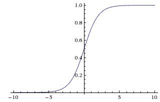
二、代价函数
线性回归:$\displaystyle J (\theta)={1 \over m}\sum_{i=0}^m {1 \over 2}(h_\theta (x_i)-y_i)^2$
逻辑回归:$cost (h_\theta (x), y)=
\begin {cases}
-log (h_\theta (x)), & \text {if $y=1$} \\
-log (1-h_\theta (x)), & \text {if $y=0$}
\end {cases}$
$cost (h_\theta (x), y)=-y \, log (h_\theta (x))-(1-y) log (1-h_\theta (x))$
$\displaystyle J (\theta)=-{1 \over m}[\sum_{i=0}^m \, log (h_\theta (x))-(1-y) log (1-h_\theta (x))]$
梯度下降法
$Repeat$
$\lbrace$
$\quad \theta_j := \theta_j - \alpha {\partial \over \partial \theta_j} J (\theta)$
$\rbrace$
$cost (h_\theta (x), y)=-y \, log (h_\theta (x))-(1-y) log (1-h_\theta (x))$
$\displaystyle {\partial cost (h_\theta (x), y) \over \partial \theta}$
$\displaystyle =-{1 \over m} \sum_{i=0}^m ({y \over h_\theta (x)} - {(1-y) \over 1-h_\theta (x)}) {\partial h_\theta (x) \over \partial \theta}$
$=\displaystyle =-{1 \over m} \sum_{i=0}^m ({y \over h_\theta (x)} - {(1-y) \over 1-h_\theta (x)}) h_\theta’(x) x$
$=\displaystyle {1 \over m} \sum_{i=0}^m {h_\theta’(x) x \over h_\theta (x)(1-h_\theta (x))}(h_\theta (x) - y)$
$=\displaystyle {1 \over m} \sum_{i=0}^m x (h_\theta (x)-y)$
三、多分类
可以分别做若干次二分类
四、逻辑回归正则化
代价函数:$\displaystyle J (\theta)=-{1 \over m}[\sum_{i=0}^my \, log (h_\theta (x))-(1-y) log (1-h_\theta (x))] + {\lambda \over 2m} \sum_{i=0}^m \theta_j^2$
五、正确率 / 召回率 / F1 指标
正确率 Precision:检索出来的条目有多少是正确的
召回率 Recall:正确的条目有多少被检索出来了
$\displaystyle F_1 值 ={2 \times {正确率 + 召回率 \over 正确率 \times 召回率}}$
正确率和召回率有时候是矛盾的,所以在不同场合需要自己判断正确率或是召回率的重要性
$\displaystyle F_\beta={(1+\beta^2) \times {正确率 + 召回率 \over (\beta^2 \times 正确率) \times 召回率}}$
六、sklearn 实战逻辑回归
1 | logistic = linear_model.LogisticRegression () |
七、sklearn 实战非线性逻辑回归
1 | logistic = linear_model.LogisticRegression () |
机器学习算法系列
机器学习算法 —(1)线性回归和非线性回归
机器学习算法 —(2)逻辑回归
机器学习算法 —(3)神经网络
机器学习算法 —(4)KNN
机器学习算法 —(5)决策树
机器学习算法 —(6)集成学习
机器学习算法 —(7)贝叶斯算法
机器学习算法 —(8)聚类算法
机器学习算法 —(9)主成分分析 PCA
机器学习算法 —(10)支持向量机 SVM